


Being able to have a clear idea of the performance of glass furnaces is not an easy aspect, due to a series of characteristics such as pollution and energy, for example. In this article we are taken through the tests carried out on 20 furnaces to obtain their energy consumption levels.
A. Bussolati, M. Marchegiani, L. Tosini
Bormioli Rocco
A. Mola
SGRPRO
E. Cattaneo
Stara Glass
One of the most challenging aspects of such an energy-intense sector as glass melting is the classification of the various furnaces’ performance in terms of energy, pollution and other aspects, as comparison between the different furnaces, and as an evaluation of one furnace’s performance over time.
This is a problem with different valences and different points of view that enable, on the one hand, to verify design conditions (and if necessary improve them) with consequences on the design sector and on optimizing and stabilizing conduction, with benefits also on the quality of the glass produced.
For example, the correlation between furnace consumption and other parameters such as pull or cullet utilization is known, but it is generally evaluated on a quality level and it makes the numerical comparison of furnaces that operate in different situations difficult.
GLASS FURNACES, WORKING CONDITIONS AND PERFORMANCE
It should be taken in account that, generally speaking, glass furnaces do not work in constant and stable conditions; they are, in fact subject to pull changes, colour, cullet and energy variations, not to mention the controlled and uncontrolled variability connected to the batch, in term of composition and humidity.
The furnace operator compensates these variations by acting on control parameters such as fuel flow, boosting power and/or distribution, batch-charging strategy, etc., aiming at ‘partial goals’ typically of a thermal nature, such as bottom temperature, crown temperature or throat glass temperature.
Most running furnaces are set to collect the values of all parameters influencing production, thus providing the possibility of functional monitoring that compares the actual performance with the foreseen and budgeted one. This comparison has to be extended to the dimension of time, since all thermal systems suffer from a non-completely predictable aging that affects the consumption significantly.
Specific consumption
Considering the most elementary measure of furnace energy performance, specific consumption [MJ/ton], we can see how this evolves depending on many parameters, not all under control.
For example, the specific consumption of a 60-tpd furnace is not comparable to a 280-tpd furnace. Other differing parameters such as cullet and boosting utilization or required quality level make different furnaces harder to compare.
It is therefore necessary to use a modelling approach to furnace energy performance, and this can be based on the evaluation of furnace heat balance, in its input and output voices.
This classification enables to quantify the result of design choices and operational settings in a more precise way. For example, the size of a furnace affects its thermal loss and, secondarily, its leakages and infiltrations.
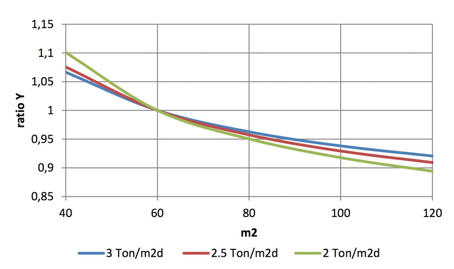
It is obvious how thermal losses, both from plain structures and thermal bridges, increase with the furnace surface, but not in a proportional way, which means that at the increase of the furnace size, the ratio between thermal loss and produced glass decreases, thus decreasing specific consumption. The more the furnace size increases, the less evident the effect of thermal loss is, as shown in Figure 2, where the specific consumption of a same production is evaluated at three different levels of specific pull for different furnace sizes.
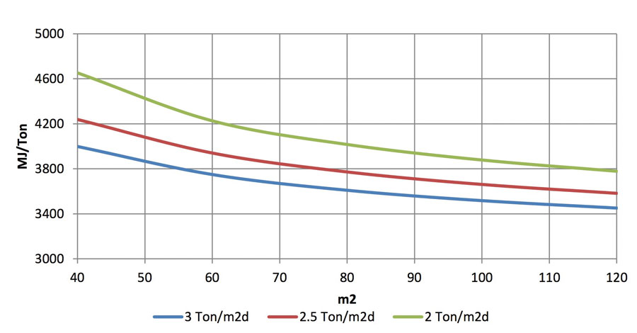
Or, if we want to analyze the situation from another point of view, we can consider that, compared to a 60 m2 furnace, a 100 m2 furnace allows a specific consumption reduction of 6.2 per cent at 3 ton/m2day and of 8.2 per cent at 2 ton/m2day as reported before.
It is important to face these aspects with an analytic approach, because the common practice of utilizing furnaces of different sizes for different productions tends to distort observations.
It is, in any case, possible to estimate an expected consumption, depending on the primary production information. This article analyzes the effect of a thermal-dynamic approach to consumption evolution by discriminating between the sensible production data and a certain unavoidable background noise, depending on the approximation of data detection and on the most obvious indeterminations characterizing every industrial (and human) process.
FURNACE COMPARISON
Twenty furnaces were analyzed during the entireness or almost of their campaigns, based on their thermal balance, and a comparison between previsions and outcomes was made. For reasons connected to data homogeneity, we decided to compare the furnaces based on their pull, cullet percentage and boosting utilization percentage, while other parameters were considered to affect the non-explained variability. Consumption was evaluated monthly, thus further feeding the uncertain part of the measure.
The first examined furnace produces domestic glass and it was followed for the 96 months of its campaign. The specific consumption is plotted with its data dispersion in Figure 4.
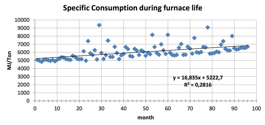
The consumption average value is 6039 MJ/ton, and the standard deviation is 884 MJ/Ton. The consumption increase during the campaign is evident and it can be described by a straight line such as the one in the figure, that displays a correlation coefficient of 0.2816.
In this case, by subtracting the variance explained by the time-trend, the standard deviation is reduced to 749 MJ/ton, and it therefore is still displaying a high margin of unexplained variation.
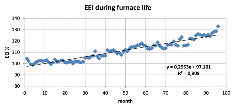
If we use modelling that considers pull, and cullet and boosting percentage, we identify an expected consumption depending on these parameters, and we relate the actual consumption to it, resulting in an Energy Efficiency Index, which is shown in pre-central terms in Figure 5.
This index, in a first approximation, does not depend on the most impacting operating conditions and it explains in the most complete way the time evolution of the energy performance, as the value R2=0.909 shows.
In statistical terms, if we plot in function of time, not consumption, with its difference with the expected value (blue line), we have a trend similar to the red one in Figure 6.
EEI = (real specific consumption) / (expected specific consumption)
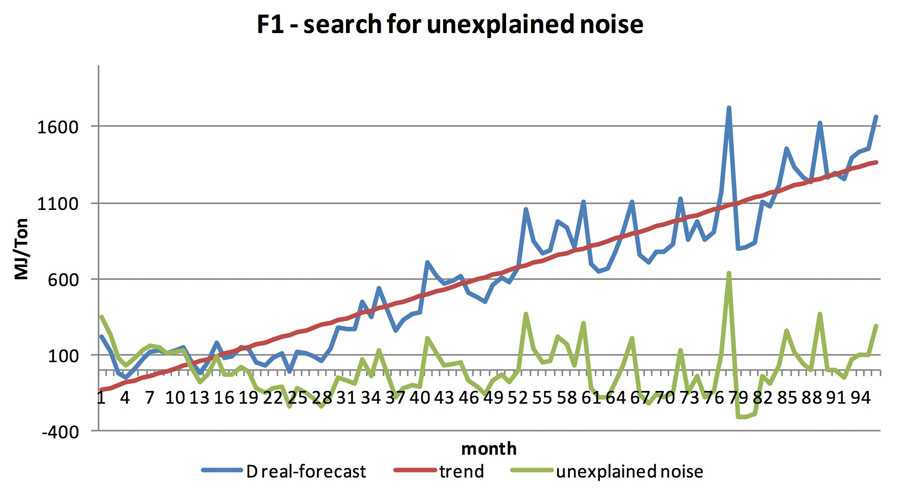
At this point, the consumption quota that is not explained by modelling or by measured aging
is represented in green, and it shows a 166 MJ/Ton average value, instead of the previous 884 MJ/Ton.
Therefore, starting from a variance of 884 MJ/Ton, we reduced it to 749 MJ/Ton by relating the data to time, and then pushed it to the indetermination of just 166 MJ/Ton by using modelling. These trends, with the variables implicit in the specific cases, can be seen in other furnaces, such as:
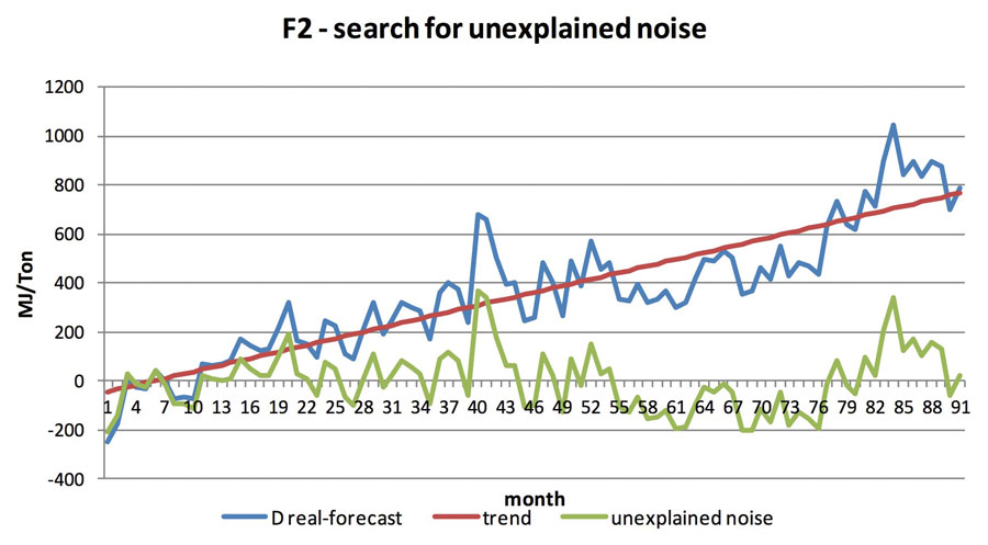
or
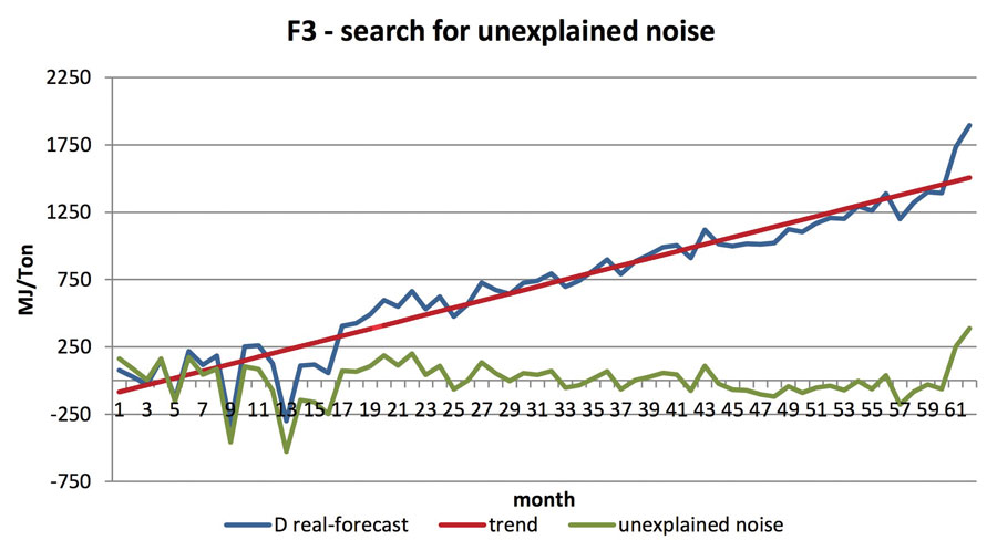
We examined 20 furnaces that present very different structural and production features, and the result is summarized in the next table.
The first column shows the basic standard deviation data related to specific real consumption. The second shows the non-explained deviance after the first data filtration using a linear relation with time. The third shows what is left unexplained after the comparison between data and model prediction, and time filtration.
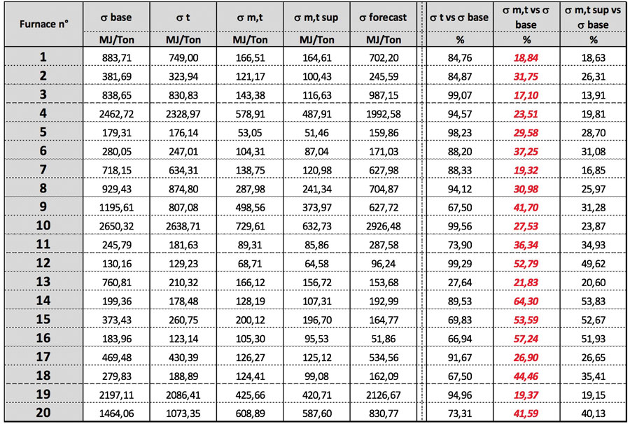
For a more in-depth analysis, we then evaluated a possible correlation of the left residual with the model parameters (pull, cullet, boosting) on a statistic base. This further correlation necessarily produces smaller residuals since it includes all previous parameters relations. (In fact, a second-degree correlation is always better than a first-degree one.) This correlation may therefore point out eventual underestimations of the weight of some of the parameters of the model. We actually notice how the explicatory effect is so limited, that it does not justify any modelling complication that do not appear proportioned to the obtainable results.
In the last three columns this data is reported as percentage.

ADDITIONAL OBSERVATIONS
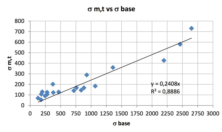
Other observations can be made. For example, it is useful to look at the deviance not just in percentage terms, but also in absolute ones. If we graph the unexplained deviance as a function of the initial one we see how well it responds to a linear model (with obvious intercepts 0.0) with a slope of 0.24 and a correlation index of 0.89. This means that this approach confirms that, on average, 76 per cent of the deviance can be explained and removed basing on a model that considers the three main production parameters (pull, cullet, boosting), and the furnace age.
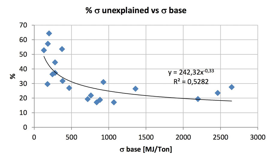
We also notice that, for limited values of the base deviance, corresponding to very-stable operating conditions, the percentage of non-explained deviance appears to be limited.
We can say that, below 500 MJ/ton, the non-explained values are above 30 per cent, while beyond this value they decrease to 20-25 per cent.
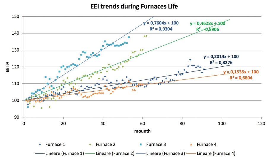
An EEI-based evaluation method enables not only to monitor the performance of the melting furnace when the operating conditions change, but also to better appreciate and compare the aging trend on the different furnaces.
Figure 12 indicated clearly the evolution of the energy efficiency index of four furnaces that shows, the aging dynamics in a standardized way, starting from a value of 100, in four specific situations that respectively express an aging rate of 0.15, 0.2, 0.46 and 0.76 on a monthly basis.
CONCLUSIONS
In conclusion, the above confirms that, as a follow up of a thermal balance, we are able to better characterize the consumption of the single furnace.
Through the parameters of conduction and through the modelling we are able to:
- Evaluate if real consumption aligned to the foreseen or if over-consumption are observed. In this case, the causes must be sought and focused on (for example, they might depend on regenerator clogging, infiltrations, etc.);
- Compare specific consumption of furnaces with different surface, pull, cullet and electric boosting utilization;
- Estimate the evolution of consumption over time, evaluating and quantifying the aging dynamics;
- Assess the expected consumption of a furnace from the main production parameter data (pull, cullet and electrical energy utilization).
![]()
Bormioli Rocco SpA
www.bormiolirocco.com
![]()
Stara Glass – Hydra Group
www.staraglass.com
![]()
SGRPRO